Code
import numpy as np
import matplotlib.pyplot as plt
from sklearn.ensemble import IsolationForest
from datasets import load_dataset
from PIL import Image

# Load the dataset
dataset = load_dataset('Bingsu/Cat_and_Dog') Anomalies are defined as events that deviate from the standard; they occur rarely and do not follow the established pattern.
In machine learning, anomaly detection, also known as outlier detection, is the identification of rare data points which raise suspicions by differing significantly from the majority of the data. Anomalies can be indicative of issues such as bank fraud, structural defects, medical problems, or errors in a text.
Examples of anomalies include:
Large dips and spikes in the stock market due to world events
Defective items in a factory/on a conveyor belt
Contaminated samples in a lab
Identifying unusual patterns that might indicate fraudulent activity
Detecting anomalies in patient data that could indicate medical issues
Unsupervised vs Supervised Detection:
Unsupervised Detection: Most common in anomaly detection. Techniques include autoencoders and clustering algorithms, for scenario when the nature of anomalies is not known a priori.
Supervised Detection: Classification models can be trained to detect anomalies with labeled data. It’s is not a recommended for real-world data is more noisy and human can miss some aspects of data when labeling it.
Semi-supervised Learning: Involves training on a large amount of unlabeled data and a small amount of labeled data.
Anomaly detection in computer vision focuses on identifying abnormal patterns or objects in visual data that do not conform to expected norms.
Isolation Forest is a type of ensemble algorithm and consist of multiple decision trees used to partition the input dataset into distinct groups of inliers. It is good for high-dimensional data like image data and is based on the principle that anomalies data points that are “isolated” in the sense that they are rare and different in terms of pixel values.
Let’s try if a human is better at distinguish cats than a “robot” using the Isolation Forest. Anomalies will be those points that have a shorter average path length in the trees of the forest.
We load the cats_vs_dogs dataset to start.
import numpy as np
import matplotlib.pyplot as plt
from sklearn.ensemble import IsolationForest
from datasets import load_dataset
from PIL import Image
# Load the dataset
dataset = load_dataset('Bingsu/Cat_and_Dog') Preprocess the dataset to get a majority of dogs and a few of cats as anomalies.
from datasets import concatenate_datasets
data = dataset['train']
cats = data.filter(lambda x: x['labels']==0)
dogs = data.filter(lambda x: x['labels']==1)
data = concatenate_datasets([cats.shuffle(seed=1).select(range(100)), dogs.shuffle(seed=0).select(range(900))])
data = data.shuffle(seed=0)
We also preprocess the images to get array representations of pixels for fitting the model.
def preprocess_image(image):
    # convert the input image to grayscale
    #image = image.convert('L')
    image = image.resize((64, 64))  # Resize to 64x64
    return np.array(image).flatten()  # Flatten the image

# Preprocess the images
images = np.array([preprocess_image(item['image']) for item in data])
Apply Isolation Forest to the dogs dataset and plot out some anomalies to see if they are cats!
# Applying Isolation Forest
iso_forest = IsolationForest(n_estimators=100, contamination=0.1)  # contamination is an estimate of the proportion of outliers
anomalies = iso_forest.fit_predict(images)

# Identifying the indices of anomalies
anomaly_indices = np.where(anomalies == -1)[0]

# Plot some of the detected anomalies
fig, axs = plt.subplots(1, 4, figsize=(15, 3))
for i, idx in enumerate(anomaly_indices[:4]):
    axs[i].imshow(images[idx].reshape(64, 64,3), cmap='gray')
    axs[i].axis('off')
    axs[i].set_title(f'Anomaly {i+1}')

plt.show()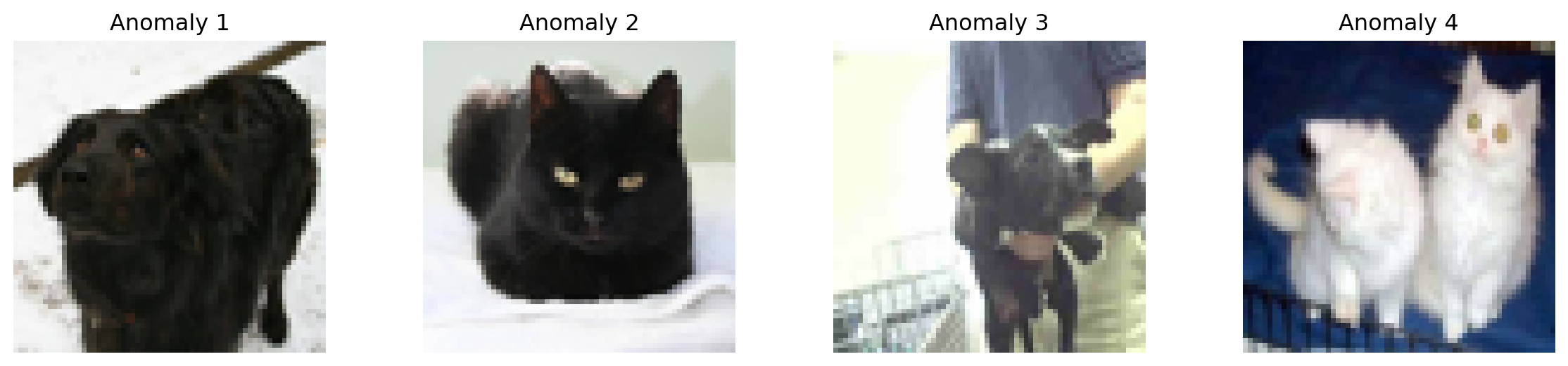
We can see the detection is not very good, the model seems to only capture the black and white color as the anomalies, which might not always hold true for all types of anomalies in image data.
Thus, we could try some more complex models such as Autoencoders, which use neural networks designed to compress and then reconstruct input data, often used to detect anomalies by comparing the reconstruction error.
We looked at twitter topic modeling with HDBSCAN clustering in the Clustering blog. We removed outliers at the time, now let’s plot the outliers too. Cluster -1 in HDBSCAN clusters is the collection of outliers.
import numpy as np
import pandas as pd
from langchain.embeddings.openai import OpenAIEmbeddings
from dotenv import load_dotenv

load_dotenv()

import hdbscan

# For plotting
from matplotlib import offsetbox
import matplotlib.pyplot as plt
import seaborn as sns
from sklearn.manifold import TSNE

dataset = load_dataset("cardiffnlp/tweet_topic_single", split="train_2021")
embeddings = OpenAIEmbeddings(chunk_size=1000).embed_documents(dataset["text"])

tensor=np.array(embeddings)

tsne = TSNE(random_state = 1, n_components=2,verbose=0).fit_transform(tensor)

cluster = hdbscan.HDBSCAN(min_cluster_size=20, prediction_data=True).fit(tsne)

df = pd.DataFrame({
    "tweet": dataset["text"],
    "label": dataset["label_name"],
    "cluster": cluster.labels_,
})

plt.scatter(tsne[:, 0], tsne[:, 1],s=5, c=df["cluster"])
plt.gca().set_aspect('equal', 'datalim')
plt.colorbar()
plt.title('Tweets topic t-SNE', fontsize=20)
Text(0.5, 1.0, 'Tweets topic t-SNE')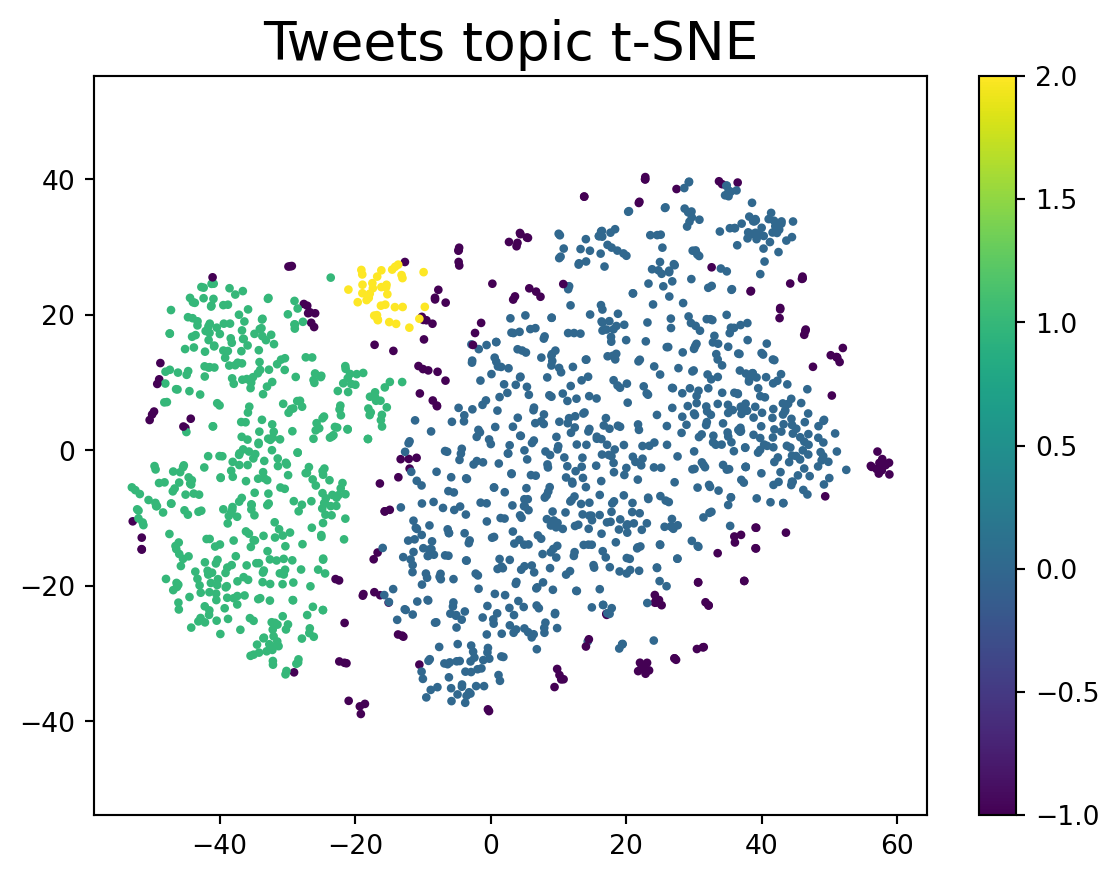
Let’s take a look at what kind of tweets are outliers
df[df["cluster"] == -1].head(5)| tweet | label | cluster | |
|---|---|---|---|
| 1 | start the 20-21 school year off POSITIVE! let’... | daily_life | -1 |
| 4 | Up with new grace, truly sorry on behalf of {@... | pop_culture | -1 |
| 30 | I spoke to ESPN about the air quality issues t... | sports_&_gaming | -1 |
| 37 | Sources Re Air Quality: {@Dallas Cowboys@} (pi... | sports_&_gaming | -1 |
| 38 | Check out what I just added to my closet on Po... | daily_life | -1 |